[ticalc.org 펌] Gamma & Zeta function +more. 감마 제타 함수 외
-

- 2025.10.29 - 12:13 2025.10.29 - 11:04 2236 2
원본 출처
https://www.ticalc.org/archives/files/fileinfo/415/41529.html
Gamma ver 1.3. by Mauritz Blomqvist (for the Nspire CAS)
This small package does contain implementations of some various special functions like the Gamma function and the Reimann Zeta function.
Some of the functions will return exact values in special cases.
The algorithms are based on information from the Gnu C Scientific library, from NUMERICAL RECIPES, The Art of Scientific Computing, Third Edition, from http://mathworld.wolfram.com/, from various documents mentioned in the files and from own ideas and algorithms.
This version is greatly extended from the version 1.1. In that version I also forgot to set some variables to LibPriv, which meant that some functions did not work outside this library. The basic difference between this version and version 1.2 is the addition of functions related to the Riemann Zeta function.
A suggestion is that you place this in a map under MyLib. Do not forget to update the library access.
Please report errors or comments to me at MauritzTortoise…telia.com where …=@.
설명 번역 :
✦ Mauritz Blomqvist의 감마 버전 1.3 (현재 CAS 및 비 CAS 버전 제공)
이 작은 패키지에는 감마 함수, 리만 제타 함수 및 관련 함수와 같은 다양한 특수 함수의 구현이 포함되어 있습니다. 대부분의 함수에 대해 복소수 인수를 처리할 수 있습니다.
gamma.tns 파일은 CAS용이고 gammanc.tns는 비 CAS용입니다. CAS 버전은 gamma(7/2)와 같은 일부 특수한 경우에 정확한 값을 반환합니다.
함수 소개 번역
✦ Gamma and related functions
gamma(z)
이 작은 패키지는 감마 함수 계산을 위한 란초스 근사(Lanczos approximation) 구현을 포함합니다. 실수 및 복소수 입력 모두에 대해 상당히 정확한 값을 반환합니다.
수식은 다음과 같습니다:
Γ(z)=gamma(z)≡∫(t^(z-1)*e^(-t),t,0,∞)
실수부와 허수부 모두 평균 0, 표준편차 30인 정규분포를 따르는 1000개의 숫자로 테스트한 결과, 상대 오차는 대부분 실수부와 허수부 모두에서 1E-10 이하 수준이었습니다. 가장 큰 상대 오차는 약 4E-8이었습니다.
이 함수는 양의 정수와 ½의 배수에 대해 정확한 값을 반환합니다.
gamma(3.5) 3.323350970447
gamma(((7)/(2))) ((15*√(π))/(8))
gamma(3.) 2.
gamma(3) 2
gamma(((−7)/(2))) ((16*√(π))/(105))
gamma(1+2i) 0.15190400267+0.019804880162*i
gamma(30) 8841761993739701954543616000000
gamma(30.) 8.84176199374E30
------
lngamma(z)
감마의 자연로그입니다. 감마 함수에 큰 인수가 필요할 때 사용할 수 있습니다.
아래 답변은 최소 유효 숫자의 한 단위 내에서 정확합니다.
lngamma(10000) 82099.7174964
일반 감마 함수는 이처럼 큰 입력을 처리할 수 없습니다.
ln(gamma(10000)) ln(9999!)
lngamma(20) ln(5773625)+2*ln(145152)
------
digamma(z)
감마의 로그 미분입니다. 즉, (d/dz)(lngamma(z))입니다.
digamma(1) −0.577215664901
이것은 -γ(오일러-마스케로니 상수)입니다.
-γ −0.577215664902
------
dergamma(z)
감마의 미분입니다.
dergamma(10) 817115.979521
------
doublefactorial(n)
이중 계승(double factorial)입니다. n!!=n*(n-2)*....
doublefactorial(8) 384
doublefactorial(7) 105
------
lowerigamma(a,z)
하 불완전 감마 함수(lower incomplete gamma)를 계산합니다:
γ(a,z)≡∫(t^(a-1)*e^(-t),t,0,z).
------
upperigamma(a,z)
상부 불완전 감마 함수(upper incomplete gamma)를 계산합니다:
Γ(a,z)≡∫(t^(a-1)*e^(-t),t,z,∞).
upperigamma(3,2) 10*e^(−2)
lowerigamma(3,2)+upperigamma(3,2) 2.
upperigamma(10,((3)/(2)))
((832670037*e^(((−3)/(2))))/(512))
------
p(a,z)
정규화된 하부 불완전 감마 함수(regularized incomplete lower gamma)를 계산합니다.
((γ(a,z))/(Γ(a))).
------
q(a,z)
정규화된 상부 불완전 감마 함수(regularized incomplete upper gamma)를 계산합니다.
((Γ(a,z))/(Γ(a))).
------
invp(pr,a)
p의 역함수입니다.
invp(p(2.2,3.4),2.2) 3.4
------
erf(z)
오차 함수(error function)입니다. 불완전 감마 함수를 기반으로 하며, 내장된 normCdf 함수를 기반으로 하는 것보다 정확도가 더 높습니다.
erf(1.3) 0.934007944941
2*normCdf(−∞,1.3*√(2),0,1)-1 0.934008064885
첫 번째 결과는 올바르게 반올림된 답, 즉 12개의 유효 숫자를 반환합니다. 마지막 결과는 6개의 유효 숫자만 반환합니다.
------
errfc(z)
여오차 함수(complementary error function)입니다.
------
inverf(x)
오차 함수의 역함수입니다.
erf(inverf(0.5)) 0.5
------
beta(x,y)
베타 함수입니다.
------
gammaintegrand(z,t)
감마 함수의 정의에 사용되는 피적분 함수입니다.
gammaintegrand(z,t) t^(z-1)*e^(−t)
------
m(a,b,z)
쿠머(Kummer)의 합류 초기하 함수(confluent hypergeometric function)입니다.
이는 γ(a,x)=((z^(a)*e^(−z)*m(1,a+1,z))/(a)) 관계식을 통해 아래 불완전 감마 함수를 계산하는 다른 방법을 제공합니다.
이것은 lowerigammam(a,z)으로 구현되어 있습니다.
이것은 또한 복소수 인수에 대한 불완전 감마를 계산하는 데 사용될 수 있습니다.
lowerigammam(2,3+2i ) 0.992332417697+0.222522474629*i
lowerigamma와 upperigamma에서 인수가 복소수일 때 사용됩니다.
✦ 몇 가지 관련 확률 함수
먼저 감마 분포와 관련된 몇 가지 함수입니다.
gammapdf(x,k,θ)
: 감마 확률 밀도 함수(Gamma Probability Density Function)
gammacdf(x,k,θ)
: 감마 누적 분포 함수(Gamma Cumulative Distribution Function)
invgammacdf(pr,k,θ)
: 역 감마 누적 분포 함수(Inverse Gamma Cumulative Distribution Function)
------
ncdf(x,μ,σ)
NormCdf(−∞,x,μ,σ)와 동일하지만, 정확도가 더 높습니다 (그리고 더 느립니다).
오차 함수 erf(z)를 사용하여 계산되며, 이는 다시 불완전 감마 함수를 사용합니다.
일반적인 입력값에 대해 내장 함수는 약 8개의 유효 숫자를 제공하는 반면, 이 함수는 기본적으로 최소 유효 숫자의 몇 부분에 해당하는 오차만을 가집니다.
------
invn(x,μ,σ)
InvNorm(x,μ,σ)와 동일하지만, 정확도가 더 높습니다 (그리고 더 느립니다).
✦ 리만 제타 함수 및 관련 함수
zeta(s)
이 함수는 리만 제타 함수를 계산하며, 보와인(Borwein) 알고리즘을 기반으로 합니다.
정수에 대해 다음 식이 성립합니다.
ζ(s)=∑(((1)/(k^(s))),k,1,∞)
그리고 s=1에서의 극점(pole)을 제외한 전체 복소 평면으로 확장하면 다음과 같습니다.
ζ(s)=((1)/(Γ(s)))*∫(((t^(s-1))/(e^(t)-1)),t,0,∞)
실제로 이 수식으로 계산할 수도 있지만, 매우 느리고 정확도도 매우 낮을 것입니다.
------
zetazero(t)
이 함수는 추측값 t 근방의 임계선(critical line) 상에서 근(root)을 찾으려고 시도합니다.
이것이 첫 번째 근입니다:
zetazero(14) 14.1347251417
zeta(0.5+14.1347251417*i) 4.E−12-3.E−11*i
즉, 0에 매우 가깝습니다.
------
rszeta(s)
이 함수 또한 리만 제타 함수를 계산하지만, 정확도는 낮지만 더 빠르며, 주로 임계대(critical strip)에서 사용하기 위한 것입니다. 리만-지겔(Riemann-Siegel) 공식을 사용합니다.
------
eta(s)
디리클레 에타 함수(Dirichlet Eta function) 또는 교대 제타 함수(alternate zeta function)입니다.
ε(s)=∑((((−1)^(k-1))/(k^(s))),k,1,∞)
------
sterl2(n,k)
제2종 스털링 수(Sterling numbers of the second kind)입니다. n개의 원소를 가진 집합을 k개의 비어있지 않은 집합으로 분할하는 방법의 수입니다.
------
bernoulli(n)
이 함수는 제2종 스털링 수를 사용하여 다소 비효율적인 방식으로 n번째 베르누이 수를 계산합니다.
------
harm(z)
이 함수는 조화 합(harmonic sum)을 반환합니다. 100 미만의 양의 정수에 대해서는 정확한 답을 반환합니다. 다른 값에 대해서는 디감마(digamma) 함수를 사용하여 매우 정확한 근사값을 계산합니다.
이 패키지에는 다음 함수도 포함되어 있습니다:
sgn(x)
내장된 부호 함수(signum function)와 달리, 이 함수의 sgn(0)은 0을 반환합니다.
fib(z)
피보나치 수열의 수를 반환합니다. 이 함수는 복소수 영역으로 확장되었습니다.
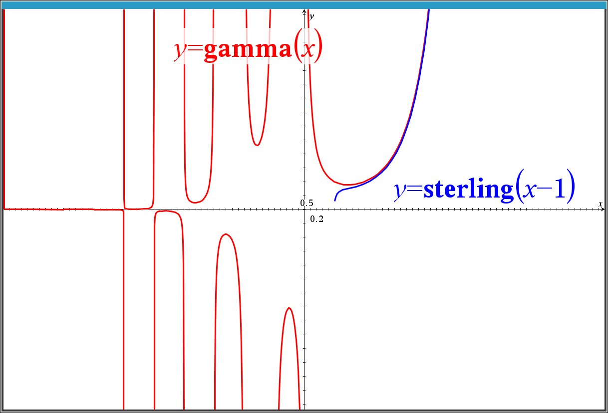
sterling(x)
계승(factorial)에 대한 스털링 근사(Sterling approximation)입니다.
오일러-감마 상수
γ=0.57721566490153
-
25
댓글2
-
세상의모든계산기
500! 의 십진수 근사값 확인
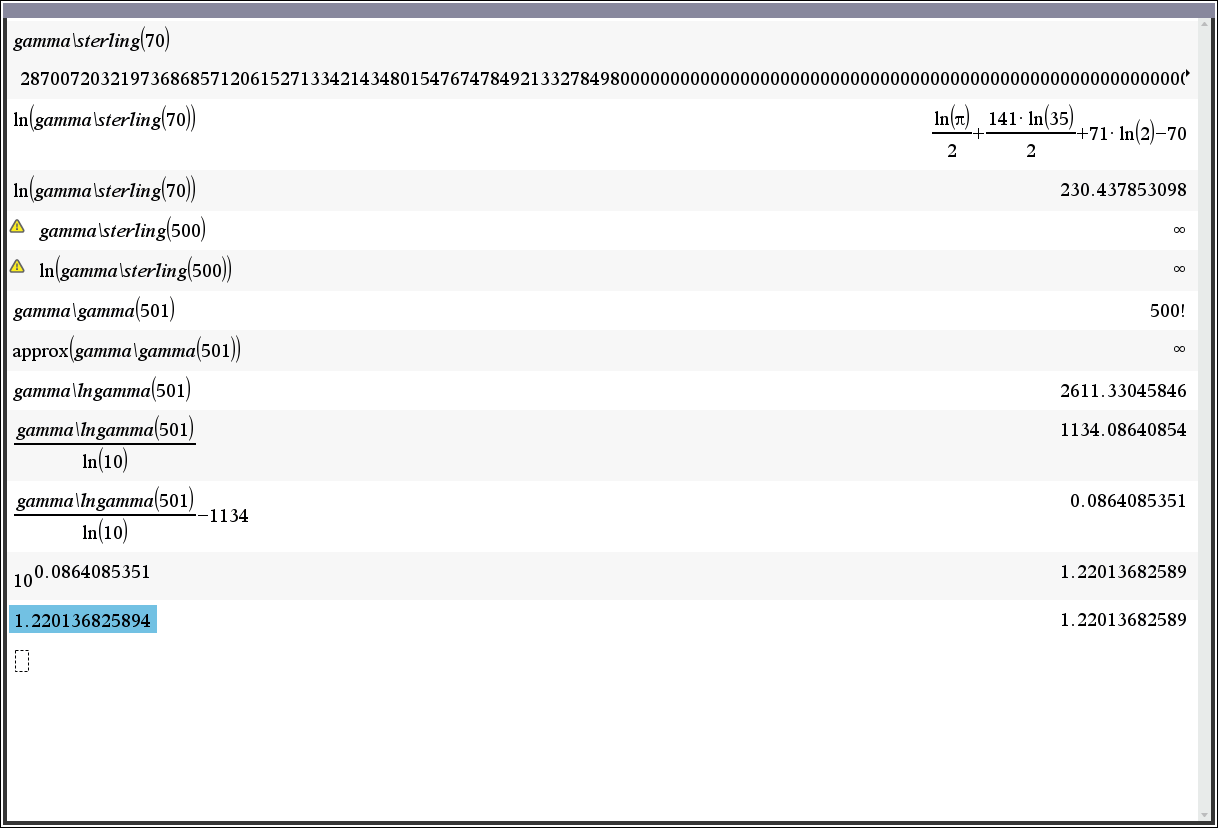
500! = 1.22013682599111006870123878542304692625357434280319284219241358838 × 10^(1134) (참값, 울프람 알파)
세상의모든계산기 님의 최근 댓글
아 그렇네요. 감사합니다. ^^ 2026 04.28 정적분 구간에 미지수가 있고, solve 를 사용할 수 없을 때 그 값을 확인하려면? https://allcalc.org/57087 `SOLVE` 기능 내에 `∫(적분)` 기호를 사용할 수 없을 때 뉴튼-랩슨법을 직접 사용하는 방법 2026 04.15 뉴턴-랩슨 적분 방정식 시각화 v1.0 body { font-family: 'Pretendard', -apple-system, BlinkMacSystemFont, "Segoe UI", Roboto, Helvetica, Arial, sans-serif; display: flex; flex-direction: column; align-items: center; background: #f8f9fa; padding: 40px 20px; margin: 0; color: #333; } .container { background: white; padding: 40px; border-radius: 20px; box-shadow: 0 15px 35px rgba(0,0,0,0.08); max-width: 900px; width: 100%; } header { border-bottom: 2px solid #f1f3f4; margin-bottom: 30px; padding-bottom: 20px; } h1 { color: #1a73e8; margin: 0 0 10px 0; font-size: 1.8em; } p.subtitle { color: #5f6368; margin: 0; font-size: 1.1em; } .equation-box { background: #f1f3f4; padding: 15px; border-radius: 10px; text-align: center; margin-bottom: 30px; font-size: 1.3em; } canvas { border: 1px solid #e0e0e0; border-radius: 12px; background: #fff; width: 100%; height: auto; display: block; } .controls { margin-top: 30px; display: flex; gap: 15px; align-items: center; justify-content: center; flex-wrap: wrap; } button { padding: 12px 25px; border: none; border-radius: 8px; background: #1a73e8; color: white; cursor: pointer; font-weight: 600; font-size: 1em; transition: all 0.2s; box-shadow: 0 2px 5px rgba(26,115,232,0.3); } button:hover { background: #1557b0; transform: translateY(-1px); box-shadow: 0 4px 8px rgba(26,115,232,0.4); } button:active { transform: translateY(0); } button.secondary { background: #5f6368; box-shadow: 0 2px 5px rgba(0,0,0,0.2); } button.secondary:hover { background: #4a4e52; } .status-badge { background: #e8f0fe; color: #1967d2; padding: 8px 15px; border-radius: 20px; font-weight: bold; font-size: 0.9em; } .explanation { margin-top: 40px; padding: 25px; background: #fff8e1; border-left: 5px solid #ffc107; border-radius: 8px; line-height: 1.8; } .explanation h3 { margin-top: 0; color: #856404; } .math-symbol { font-family: 'Times New Roman', serif; font-style: italic; font-weight: bold; color: #d93025; } .code-snippet { background: #202124; color: #e8eaed; padding: 2px 6px; border-radius: 4px; font-family: monospace; } 📊 Newton-Raphson 적분 방정식 시뮬레이터 미분적분학의 기본 정리(FTC)를 이용한 수치해석 시각화 목표 방정식: ∫₀ᴬ (2√x) dx = 20 을 만족하는 A를 찾아라! 계산 시작 (A 추적) 초기화 현재 반복: 0회 💡 시각적 동작 원리 (Newton-Raphson & FTC) Step 1 (오차 측정): 현재 A까지 쌓인 파란색 면적이 목표치(20)와 얼마나 차이나는지 계산합니다. Step 2 (FTC의 마법): 면적의 변화율(미분)은 그 지점의 그래프 높이 f(A)와 같습니다. Step 3 (보정): 다음 A = 현재 A - (면적 오차 / 현재 높이) 공식을 사용하여 A를 이동시킵니다. 결론: 오차를 현재 높이로 나누면, 오차를 메우기 위해 필요한 가로 길이(ΔA)가 나옵니다. 이 과정을 반복하면 정답에 도달합니다! const canvas = document.getElementById('graphCanvas'); const ctx = canvas.getContext('2d'); const iterText = document.getElementById('iterText'); // 수학 설정 const targetArea = 20; const f = (x) => Math.sqrt(x) * 2; // 피적분 함수 f(x) = 2√x const F = (x) => (4/3) * Math.pow(x, 1.5); // 정적분 결과 F(x) = ∫ 2√x dx = 4/3 * x^(3/2) let A = 1.5; // 초기값 let iteration = 0; let animating = false; // 그래프 드로잉 설정 const scale = 50; const offsetX = 60; const offsetY = 380; function drawGrid() { ctx.strokeStyle = '#f1f3f4'; ctx.lineWidth = 1; ctx.beginPath(); for(let i=0; i 2026 04.11 참값 : A = ±2√5 근사값 : A≈±4.472135954999579392818347 2026 04.10 fx-570 ES 입력 결과 초기값 입력 반복 수식 입력 반복 결과 2026 04.10