
- 세상의 모든 계산기 수학, 과학, 공학 이야기 수학 ()
직교 좌표계 vs 극좌표계의 시각적 비교
-

- 2024.10.30 - 15:37 2024.10.27 - 18:21 1420 4
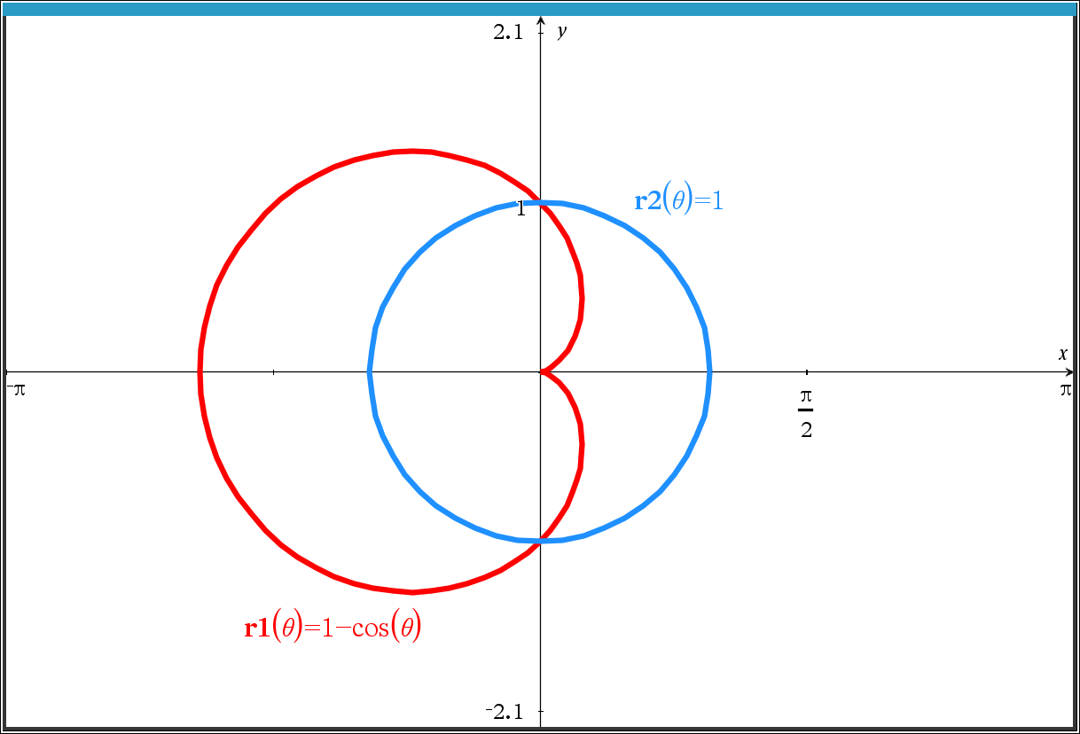
1. 두 개의 극좌표 함수가 있습니다.
2. 직교좌표계에서 표시.
Rectangular Coordinate = 카르테시안 좌표계 Cartesian coordinate system
각 축이 서로 수직(직각)으로 만남.
각 축의 값이 커지거나 작아지는 것은 일직선 위에서 발생
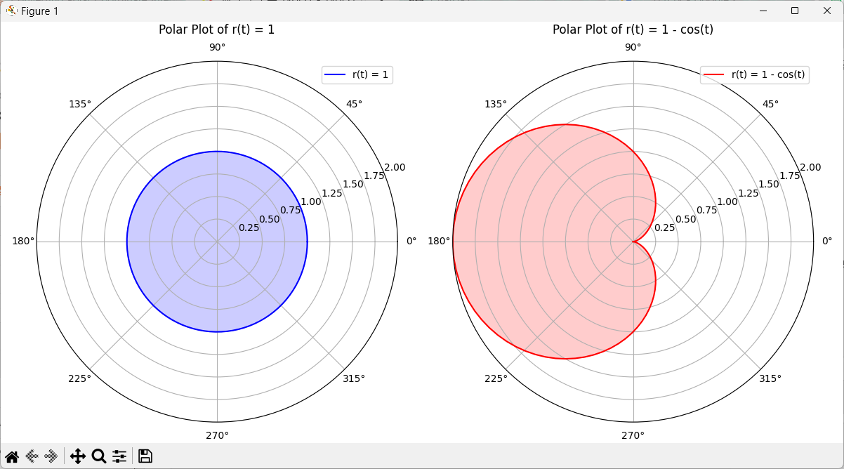
3. 극좌표계에서 표시
Polar Coordinate
import numpy as np
import matplotlib.pyplot as plt

# t의 범위 설정 (0부터 2π까지)
t = np.linspace(0, 2 * np.pi, 100)

# 극좌표 함수 정의
r1 = np.ones_like(t)  # r(t) = 1
r2 = 1 - np.cos(t)    # r(t) = 1 - cos(t)

# 극좌표 그래프 그리기
fig = plt.figure(figsize=(12, 6))

# r(t) = 1 그래프
ax1 = fig.add_subplot(121, projection='polar')
ax1.plot(t, r1, label='r(t) = 1', color='b')
ax1.fill(t, r1, color='blue', alpha=0.2)  # 그래프 아래 영역 채우기
ax1.set_title('Polar Plot of r(t) = 1', va='bottom')
ax1.set_ylim(0, 2)  # 반지름 범위 설정
ax1.legend()

# r(t) = 1 - cos(t) 그래프
ax2 = fig.add_subplot(122, projection='polar')
ax2.plot(t, r2, label='r(t) = 1 - cos(t)', color='r')
ax2.fill(t, r2, color='red', alpha=0.2)  # 그래프 아래 영역 채우기
ax2.set_title('Polar Plot of r(t) = 1 - cos(t)', va='bottom')
ax2.set_ylim(0, 2)  # 반지름 범위 설정
ax2.legend()

# 그래프 보여주기
plt.tight_layout()
plt.show()
극좌표계의 구조
-
각도 축: 극좌표계에서tt 축(각도 축)은 원점을 기준으로 하는 방향을 나타냅니다. 각도는 일반적으로 반시계 방향으로 측정되며, 0에서 2π까지 변화합니다.
-
반지름 축: r 축(반지름)은 원점으로부터의 거리로, 특정 각도에 따라 뻗어 있습니다. 반지름은 원점에서 시작하여 외부로 나아가며, 주어진 각도 t에서의 반지름 r 값에 따라 점이 위치하게 됩니다.
-
동심원: 극좌표계는 다양한 반지름에 대해 중심이 같은 원을 그리는 "동심원" 형태로 되어 있습니다. 즉, 반지름 r의 값에 따라 같은 각도 t에서 원의 크기가 결정됩니다.
4. 비교
- 직교좌표계에서는 x축과 y축이 수직으로 만나며, 각 축이 서로의 기준을 이루는 데 반해,
- 극좌표계에서는 각도와 반지름이 서로 독립적인 성질을 가지며, 각도는 방향을, 반지름은 거리를 나타내게 됩니다.
-
25
댓글4
-
세상의모든계산기
극좌표계에서의 면적 요소 \(dA\)
1. 부채꼴 형상:
- 극좌표계에서 \(r\)와 \(\theta\)의 변화에 따라 만들어지는 면적 요소는 부채꼴의 형태를 가집니다. 그러나 이 부채꼴은 작아질수록 사각형에 가까워집니다.2. 사각형 근사:
- 부채꼴의 끝부분이 작아질 때, 이를 사각형으로 근사할 수 있습니다. 이때 사각형의 한 변은 \(dr\) (거리에 해당), 다른 변은 \(r \, d\theta\) (각도 변화에 따른 아크 길이에 해당)입니다.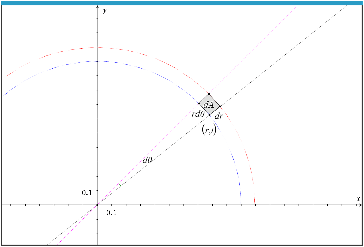
3. 면적 계산:
- 따라서 미소 면적 요소는 다음과 같이 표현할 수 있습니다:
\[
dA = r \, dr \, d\theta
\]
- 여기서 \(r \, d\theta\)는 사각형의 한 변의 길이를 나타내고, \(dr\)는 나머지 변의 길이를 나타냅니다.
- 즉, 사각형의 면적은 다음과 같이 계산할 수 있습니다:
\[
dA \approx (r \, d\theta) \cdot (dr) = r \, dr \, d\theta
\]4. 순서 변경:
- 이 면적 요소는 \(dA = r \, dr \, d\theta\)로 쓸 수 있으며, 순서를 바꿔서도 쓸 수 있습니다. 예를 들어 \(dA = r \, dr \, d\theta\)는 \(dA = dr \cdot r \, d\theta\)와 같이 쓸 수 있습니다. 이는 곱셈의 교환 법칙에 따라 가능하며, 적분할 때에도 상관없이 사용됩니다. -
세상의모든계산기
극좌표 함수의 형태로 나타나는 이중적분
극좌표 함수에서 \(dA = r \, dr \, d\theta\) 형태로 나타낼 수 있는 이중적분 \(\int \int f(r, \theta) \, r \, dr \, d\theta\)는 면적을 계산하는 방식입니다.
이 계산식에서 \(r\)과 \(\theta\)의 변화에 따른 미소 면적의 총합으로 이해할 수 있습니다.
이중적분의 의미
1. 미소 면적의 총합:
- 극좌표계에서 \(dA\)는 미소 면적 요소를 나타냅니다. \(r\)이 변화하고, \(\theta\)도 변화할 때, 각 미소 면적 \(dA\)를 모두 합산하여 전체 면적을 구하는 것이 이중적분의 목적입니다.
- 즉, \(\int_0^{\theta_{\text{max}}} \int_0^{r_{\text{max}}} f(r, \theta) \, r \, dr \, d\theta\)와 같이 표현되는 이중적분은 각 \(r\)에 대한 함수 값 \(f(r, \theta)\)와 면적 요소 \(r \, dr\)를 곱한 후, 이를 \(\theta\)에 대해 적분하여 총 면적을 구하는 과정입니다.2. 변화에 따른 적분:
- \(r\)와 \(\theta\)가 각각의 구간에서 변화할 때, 그 변화에 따른 미소 면적을 구해 적분하는 것이므로, \(t\)의 총 변화(여기서는 \(\theta\)로 표현됨)에 따른 미소 면적의 총합으로 볼 수 있습니다.결론
결국, 극좌표에서의 이중적분은 각 점의 미소 면적 \(dA\)를 합산하여 전체 면적을 구하는 과정입니다.
이때 \(r \, dr \, d\theta\)는 면적 요소로 작용하며, 이는 각각의 \(r\)과 \(\theta\)의 변화에 따른 총 면적을 반영합니다.
따라서 \(\int \int f(r, \theta) \, r \, dr \, d\theta\)는 미소 면적의 총합으로 볼 수 있습니다. 잘 이해하셨습니다!
-
1
세상의모든계산기
이중적분 \(\int_0^{2\pi} \int_0^{\sin(t)} \sqrt{1 - r^2} \cdot r \, dr \, dt\)에서 \(t\)의 변화에 따라 그래프의 변화를 연속적으로 보여주면
import numpy as np
import matplotlib.pyplot as plt
from matplotlib.animation import FuncAnimation

# 설정
t_values = np.linspace(0, 2 * np.pi, 100)  # t의 변화 범위

# 그래프 초기화
fig, ax = plt.subplots(figsize=(8, 8))
ax.set_xlim(-1.5, 1.5)
ax.set_ylim(-1.5, 1.5)
ax.set_aspect('equal')
ax.set_title('Area under the curve for varying $t$')
ax.set_xlabel('$x$')
ax.set_ylabel('$y$')

# 그래프에 사용할 점과 면적 표시
line_r, = ax.plot([], [], color='blue', label='$r(t) = \sin(t)$')
ax.legend()

# 면적 다각형 리스트
area_patches = []
total_area = 0  # 총 면적 초기화
area_text = ax.text(-1.4, 1.2, f'Total Area: {total_area:.2f}', fontsize=12)

# 애니메이션 업데이트 함수
def update(frame):
    global total_area  # 총 면적을 전역 변수로 설정
    t = t_values[frame]
    r = np.linspace(0, np.sin(t), 100)  # r 값 생성
    x = r * np.cos(t)  # x 좌표
    y = r * np.sin(t)  # y 좌표

    # 면적을 나타내는 다각형 생성
    area_patch = plt.Polygon(np.column_stack((x, y)), closed=True, color='lightblue', alpha=0.5)
    ax.add_patch(area_patch)  # 다각형 추가
    area_patches.append(area_patch)  # 면적 목록에 추가

    # 면적 계산 (부채꼴 면적 계산)
    segment_area = 0.5 * (np.sin(t) ** 2) * t  # t에 따른 면적
    total_area += segment_area  # 총 면적 업데이트

    # 선 업데이트
    line_r.set_data(np.array([0, x[-1]]), np.array([0, y[-1]]))

    # 면적 합계 텍스트 업데이트
    area_text.set_text(f'Total Area: {total_area:.2f}')

    return area_patches, line_r, area_text

# 애니메이션 생성
ani = FuncAnimation(fig, update, frames=len(t_values), blit=False, repeat=False)

# 진행 표시줄 추가
progress_ax = fig.add_axes([0.15, 0.1, 0.7, 0.05])  # 위치 조정
progress_bar = plt.barh([0], [0], color='gray', height=0.1)  # 진행 표시줄
progress_ax.set_xlim(0, len(t_values))
progress_ax.set_ylim(-0.5, 0.5)
progress_ax.axis('off')  # 축 숨기기

# 진행 표시줄 레이블 추가
start_label = progress_ax.text(-1, 0, 'Start: $t=0$', fontsize=10, ha='center')
end_label = progress_ax.text(len(t_values)+1, 0, 'End: $t=2\pi$', fontsize=10, ha='center')

# 애니메이션 프레임 업데이트
def update_progress(frame):
    progress_bar[0].set_width(frame)  # 진행 표시줄 업데이트
    return progress_bar

# 진행 표시줄 애니메이션
ani_progress = FuncAnimation(fig, update_progress, frames=len(t_values), blit=False, repeat=False)

plt.show()
세상의모든계산기 님의 최근 댓글
아 그렇네요. 감사합니다. ^^ 2026 04.28 정적분 구간에 미지수가 있고, solve 를 사용할 수 없을 때 그 값을 확인하려면? https://allcalc.org/57087 `SOLVE` 기능 내에 `∫(적분)` 기호를 사용할 수 없을 때 뉴튼-랩슨법을 직접 사용하는 방법 2026 04.15 뉴턴-랩슨 적분 방정식 시각화 v1.0 body { font-family: 'Pretendard', -apple-system, BlinkMacSystemFont, "Segoe UI", Roboto, Helvetica, Arial, sans-serif; display: flex; flex-direction: column; align-items: center; background: #f8f9fa; padding: 40px 20px; margin: 0; color: #333; } .container { background: white; padding: 40px; border-radius: 20px; box-shadow: 0 15px 35px rgba(0,0,0,0.08); max-width: 900px; width: 100%; } header { border-bottom: 2px solid #f1f3f4; margin-bottom: 30px; padding-bottom: 20px; } h1 { color: #1a73e8; margin: 0 0 10px 0; font-size: 1.8em; } p.subtitle { color: #5f6368; margin: 0; font-size: 1.1em; } .equation-box { background: #f1f3f4; padding: 15px; border-radius: 10px; text-align: center; margin-bottom: 30px; font-size: 1.3em; } canvas { border: 1px solid #e0e0e0; border-radius: 12px; background: #fff; width: 100%; height: auto; display: block; } .controls { margin-top: 30px; display: flex; gap: 15px; align-items: center; justify-content: center; flex-wrap: wrap; } button { padding: 12px 25px; border: none; border-radius: 8px; background: #1a73e8; color: white; cursor: pointer; font-weight: 600; font-size: 1em; transition: all 0.2s; box-shadow: 0 2px 5px rgba(26,115,232,0.3); } button:hover { background: #1557b0; transform: translateY(-1px); box-shadow: 0 4px 8px rgba(26,115,232,0.4); } button:active { transform: translateY(0); } button.secondary { background: #5f6368; box-shadow: 0 2px 5px rgba(0,0,0,0.2); } button.secondary:hover { background: #4a4e52; } .status-badge { background: #e8f0fe; color: #1967d2; padding: 8px 15px; border-radius: 20px; font-weight: bold; font-size: 0.9em; } .explanation { margin-top: 40px; padding: 25px; background: #fff8e1; border-left: 5px solid #ffc107; border-radius: 8px; line-height: 1.8; } .explanation h3 { margin-top: 0; color: #856404; } .math-symbol { font-family: 'Times New Roman', serif; font-style: italic; font-weight: bold; color: #d93025; } .code-snippet { background: #202124; color: #e8eaed; padding: 2px 6px; border-radius: 4px; font-family: monospace; } 📊 Newton-Raphson 적분 방정식 시뮬레이터 미분적분학의 기본 정리(FTC)를 이용한 수치해석 시각화 목표 방정식: ∫₀ᴬ (2√x) dx = 20 을 만족하는 A를 찾아라! 계산 시작 (A 추적) 초기화 현재 반복: 0회 💡 시각적 동작 원리 (Newton-Raphson & FTC) Step 1 (오차 측정): 현재 A까지 쌓인 파란색 면적이 목표치(20)와 얼마나 차이나는지 계산합니다. Step 2 (FTC의 마법): 면적의 변화율(미분)은 그 지점의 그래프 높이 f(A)와 같습니다. Step 3 (보정): 다음 A = 현재 A - (면적 오차 / 현재 높이) 공식을 사용하여 A를 이동시킵니다. 결론: 오차를 현재 높이로 나누면, 오차를 메우기 위해 필요한 가로 길이(ΔA)가 나옵니다. 이 과정을 반복하면 정답에 도달합니다! const canvas = document.getElementById('graphCanvas'); const ctx = canvas.getContext('2d'); const iterText = document.getElementById('iterText'); // 수학 설정 const targetArea = 20; const f = (x) => Math.sqrt(x) * 2; // 피적분 함수 f(x) = 2√x const F = (x) => (4/3) * Math.pow(x, 1.5); // 정적분 결과 F(x) = ∫ 2√x dx = 4/3 * x^(3/2) let A = 1.5; // 초기값 let iteration = 0; let animating = false; // 그래프 드로잉 설정 const scale = 50; const offsetX = 60; const offsetY = 380; function drawGrid() { ctx.strokeStyle = '#f1f3f4'; ctx.lineWidth = 1; ctx.beginPath(); for(let i=0; i 2026 04.11 참값 : A = ±2√5 근사값 : A≈±4.472135954999579392818347 2026 04.10 fx-570 ES 입력 결과 초기값 입력 반복 수식 입력 반복 결과 2026 04.10