
- TI 89
[TI-92][TI-89] Fourier Transform Library
-

- 2024.11.19 - 00:34 2024.11.15 - 23:18 6766 8
오리지널 출처는 모르겠구요. 이곳에서 발견했습니다.
https://helpcalculator.forumfree.it/?t=7760484
파일 다운로드 : https://digilander.libero.it/fpirozzi/fourier.zip
Readme.txt
fourier
-------
Fourier version 3.20 for TI-92/TI-92II and TI-89/TI-92+
This packet contains functions to perform Fourier-/inverse Fourier-
transformation. A function, which can rewrite the output of Fourier/
iFourie to a form that, can be evaluated numerical. A function to
graph the output.
Keep the functions together in a separate folder with the name
"FOURIER" and do not create any variable in it.
Before using iFourier or Fourier set TI-92 MODE
Complex Format to RECTANGULAR
Angle to RADIAN
Exact/Approx to AUTO
You have to do these settings yourself because; the functions cannot
change the mode setting on the calculator.
The package include following programs/functions:
Help online help to programs.
Fourier Fourier transformation
iFourier inverse Fourier transformation
Plot graph expression
eval evaluate expression
Menu custom menu
Other files in the package are all sub functions or data for above functions.
--------------------- Archiving on TI-89 and TI-92+ -------------------------
All variables can be archived on the TI-89 and TI-92+. Functions and programs can also be archived, but first after they have been used one time each. If
the programs have not been run before archiving, the calculator has to
compile them each time they are used, this will slow down the execution time
of the programs.
Before archiving the programs execute following commands from the command
line in the "fourier" folder:
Help() and press 'x'
ifourier(1/w,w)
fourier(1,t)
eval(1)
plot(1,t,0)
---------------------------------------------------------------------
Help
This program will give online information about and demonstrate the
use of functions in this package. When you do not need this program
any longer just delete it and the data file "hlp".
Syntax: Help()
---------------------------------------------------------------------
Function: Fourier(f(var), var ,mode)
Transforms the expression "f(var)" from time domain to frequency domain (Fourier). This function has the ability in the most occasions to perform symbolical transformations, but not in all. It depends on the type of transform.
f(var): can be any expression, which have a Fourier transform.
var : is the name of the variable to transform normally 't', but can be any name.
mode : decide the format of the result.
Mode can be 1 or 2.
In mode 1 the result will be in Ti-92's complex format (exp(i*w) will be rewritten to cos(w)+i*sin(w)). Mode 2 is a special format, where the calculators complex 'i' will be replaced with the letter 'i'.
The results in mode 2 will be exponential functions instead of sine and cosine. The letter 'i' in the results of Fourier is the same as the complex 'i' and can always be replaced with it.
The letter 'i' and 'complex i' will be interpreted as equal.
The expression may contain constants of any kind except constants
containing the letter 's'.
Special transforms:
Unit step function (Heaviside function):
Definition: u(t-a) = 1 for t>=a else 0
Fourier(u(t - a),t,2) = pi*'Delta'(w)-i*exp(-a*i*w)/w
Dirac delta function:
Definition: 'delta'(t - a) = 1 for t=a else 0
fourier('delta'(t - a),t,2) = exp(-a*i*w)
You can get 'delta' by pressing 'green diamond' + G + D on TI-92.
signum function:
Definition: signum(t-a) = 1 for t>=a else -1
Fourier(signum(t - a),t,2) = -i*2*exp(-a*i*w)/w
Some examples:
Fourier(cos(5*t),t,1) = pi*'delta'(w-5)+pi*'delta'(w+5)
Fourier(cos(5*t)*u(t),t,1) =
i*(-1/2*(w+5))-1/(2*(w-5))+pi*'delta'(w-5)+pi*'delta'(w+5)
Fourier(1/(t-i),t,2) = 2*pi*i*exp(w)*u(-w)
---------------------------------------------------------------------
Function: iFourier(F(var), var ,mode)
Transforms the expression "F(var)" from frequency domain to time domain
(inverse Fourier).
F(var): can be any expression, which have an inverse Fourier transform.
var : is the name of the variable to transform normally 'w', but can
be any name. This function has the ability in the most occasions to
perform symbolical transformations, but not in all. It depends on the
type of transform.
mode : decide the format of the result. Mode can be 1 or 2. In mode 1
the result will be in Ti-92's complex format (exp(i*w) will be rewritten
to cos(w)+i*sin(w)). Mode 2 is a special format, where the calculators
complex 'i' will be replaced with the letter 'i'. The results in mode 2
will be exponential functions instead of sine and cosine. The letter 'i'
in the results of iFourier is the same as the complex 'i' and can always
be replaced with it.
The letter 'i' and 'complex i' will be interpreted as equal.
The expression may contain constants of any kind except constants containing the letter 's'.
Special transforms:
Unit step function (Heaviside function):
Definition: u(w-a) = 1 for w>=a else 0
iFourier(u(w - a),w,2) = 'Delta'(-t)/2+i*exp(a*i*t)/(2*pi*t)
Dirac delta function:
Definition: 'delta'(w - a) = 1 for w=a else 0
Fourier('delta'(w - a),w,2) = exp(a*i*t)/(2*pi)
You can get 'delta' by pressing 'green diamond' + G + D on TI-92.
signum function:
Definition: signum(w - a) = 1 for w>=a else -1
Fourier(signum(w - a),w,2) = i*exp(a*i*t)/(pi*t)
Some examples:
iFourier(u(w+1)-u(w-1),w,1) = sin(t)/(pi*t)
iFourier(1/(w+1)^2,w,2) = 2*t*exp(-i*t)*(2*u(-t)-1)
iFourier('delta'(w+5)+'delta'(w-5),t,1) = sin(5*t)/pi
---------------------------------------------------------------------
Function: eval(f(var))
f(var) any function containing Heaviside, dirac delta or signum
This function will replace u(var), 'delta'(var), signum(var) with a
equivalent when-functions. The letter 'i' will be replaced with the
'complex i'.
Example: eval(u(t-a))=when(t-a>=0, 1,0)
To get a numerical result out of a function containing special
functions
eval(f(var))|var=value
---------------------------------------------------------------------
Program: Plot(f(var),var,type)
This program will graph functions containing Heaviside, dirac delta or
signum. It will not change the setting of the calculator and it is
therefore up to you to manage the window settings.
f(var) any function containing Heaviside, dirac delta or signum
var variable to plot
type=0 plot the function f(var)
type=1 plot the amplitude abs(f(var))
type=2 plot phase angle(f(var))
Example:
Plot(u(t)-u(t-4),t,0) plots a pulse
Example:
Plot the amplitude of a complex function
plot(f(war),var,1)
Plot the phase
plot(f(war),war,2)
---------------------------------------------------------------------
Author: Lars Frederiksen
E-mail: LTF@POST8.TELE.DK
PS. Please do not ask for more programs.
-
25
댓글8
-
-
세상의모든계산기
주요 함수들과 그들의 역할
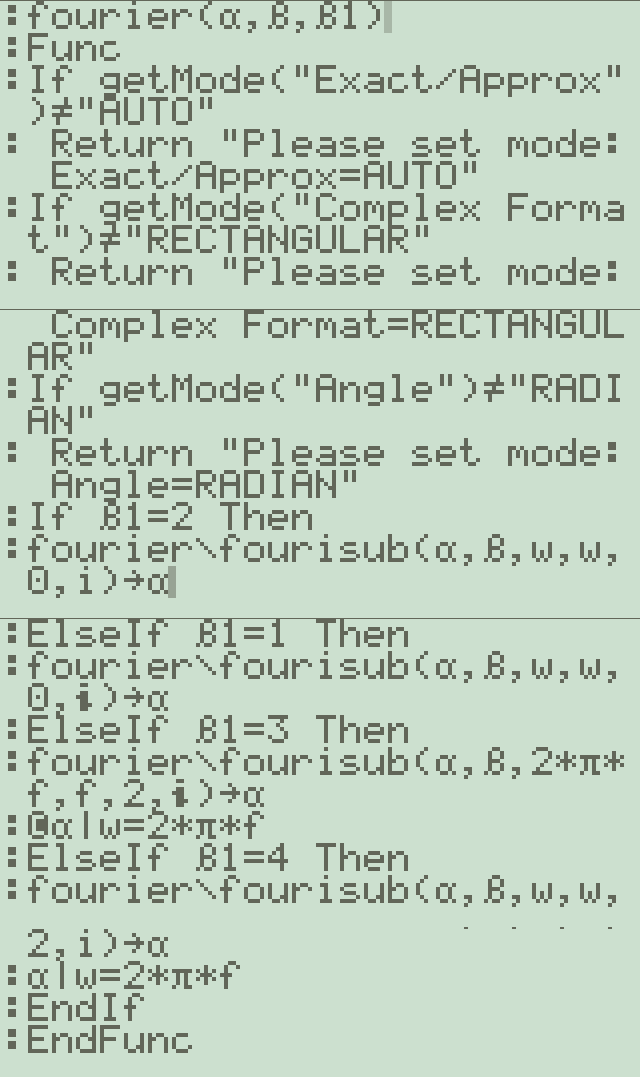
1. fourier(α,β,β1) - 메인 함수
- 모드 체크를 수행합니다 (Exact/Approx, Complex Format, Angle)
- β1 값에 따라 다른 변환 방식을 선택합니다:
- β1=1 or 2: 일반적인 푸리에 변환
- β1=3 or 4: 주파수 도메인(2πf) 변환2. fourisub(α, ββ, β1, β2, β3, βi) - 실제 변환 연산
- 복소수 형태의 푸리에 변환을 계산합니다
- 주요 처리 과정:
- 입력 함수를 파싱하여 항들을 분리
- 각 항에 대해 적분 계산
- 델타 함수(δ), 단위계단 함수(u), 부호 함수(signum) 등의 특수 함수 처리3. eval(x) - 수식 평가 함수
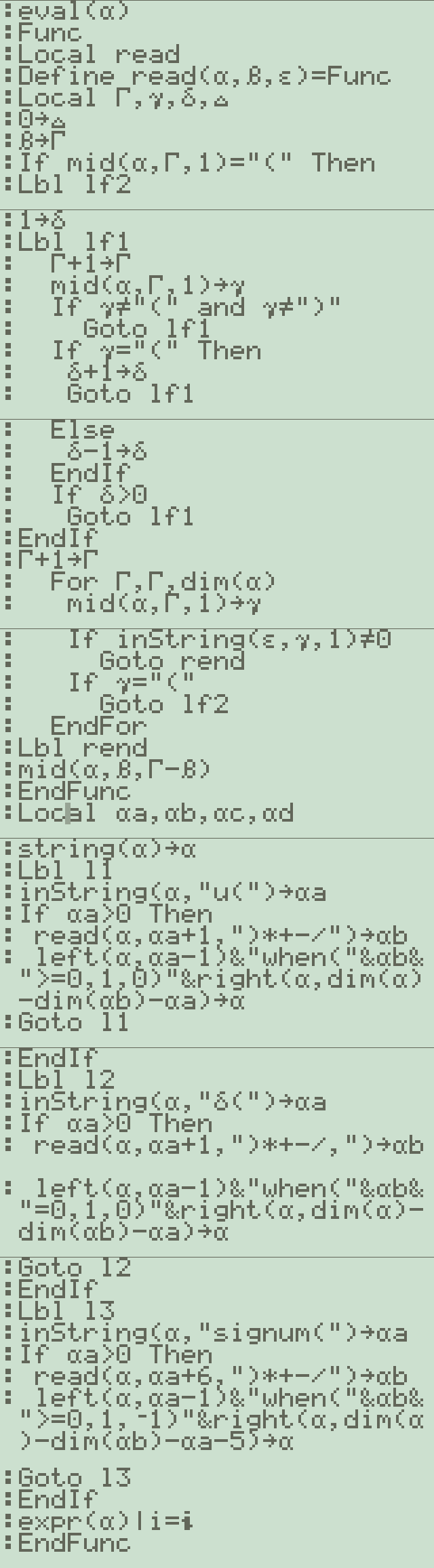
- 특수 함수들을 계산 가능한 형태로 변환:
- u(x) → when(x>=0,1,0)
- δ(x) → when(x=0,1,0)
- signum(x) → when(x>=0,1,-1) -
세상의모든계산기
예시) x(t) = e^(-at)u(t) 처리 과정
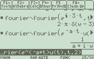
1. 함수 입력 형태와 초기 처리:
# 입력 함수 형태
α = "e^(-a*s)*u(s)" # 여기서 s는 시간 변수# eval 함수에서 단위계단 함수 변환
# "u(s)" → "when(s>=0,1,0)"
inString(α, "u(")→αa # u( 위치 찾기
read(α, αa+1,")*+-/")→αb # 인자 추출 (여기서는 's')
# 변환 결과: "e^(-a*s)*when(s>=0,1,0)"2. fourier 함수에서의 처리:
fourier(α,β,β1)
# β는 변환 파라미터
# β1은 변환 타입 (1 또는 2: 기본 푸리에 변환)# fourisub 호출
fourier\fourisub(α, β, w, w, 0, @i)→α
3. fourisub 함수에서의 주요 변환 과정:
# 1) 입력 함수 파싱
expr(αa)→αk # 수식을 파싱하여 계산 가능한 형태로 변환
getDenom(αk)→βλ # 분모 추출
getNum(αk)→βf # 분자 추출# 2) 지수함수 처리
# e^(-a*s) 부분 처리
inString(αa,"@e^",αj)→αj # 지수함수 위치 찾기
read(αa, αj,"÷−)*/")→αi # 지수 부분 추출# 3) 기본 변환쌍에 대입해 변환
# timeδ 함수와 time 함수가 실제 변환을 처리합니다
timeδ(βρ,β1,β2,β4)→αf # βρ에는 변환할 항의 정보가 담겨있습니다
# 변환 결과들은 누적됩니다
βa+αf/βλ→βa # 부분 결과들의 합산
# 특별한 경우(poles가 있는 경우) 처리
If dim(βγ)>0 Then
# βγ는 극점들의 배열
# 각 극점에 대해 처리하는 루프
For βς,1,dim(βγ)-1
Φα*(s-#("Γ"&char(ord("a")+βς)))→Φα
EndFor
# 4) 결과 조합
β3*(βa+Φw)|i^2=-1→Φw # 최종 결과 생성
수학적 계산 흐름:
1. x(t) = e^(-at)u(t)가 입력됨
2. u(t)가 when(t>=0,1,0)로 변환됨
3. 푸리에 변환 적분 적용:
X(ω) = ∫[e^(-at)u(t)e^(-jωt)]dt
4. u(t)의 특성으로 인해 적분 구간이 0에서 ∞로 변경됨
5. 적분 계산:
X(ω) = ∫[e^((-a-jω)t)]dt, from 0 to ∞
6. 적분 결과:
X(ω) = 1/(a + jω)이 과정이 코드에서 자동으로 처리되며, 특히 주목할 점은:
- 특수함수(여기서는 u(t))의 자동 변환
- 복소수 처리 (i^2=-1 조건 사용)
- 지수함수의 적분 처리
- 최종 결과의 표준화된 형태 제공이는 단순한 예시지만, 코드는 더 복잡한 함수들(예: 델타 함수, 부호 함수 등을 포함하는 함수들)도 처리할 수 있도록 설계되어 있습니다.
-
-
세상의모든계산기
function - fouriersub()
클릭해 프로그램(png) 보기 - 스크롤 주의
details

-
세상의모든계산기 님의 최근 댓글
PC 소프트웨어에서 script Editor 로 소스코드를 쉽게 복사 -> AI에게 문의/개선요청 할 수 있습니다. 잘 되거나, 잘 안되는 부분이 있으면 대댓글 남겨주세요. 2026 10.16 AI로 딸깍하니까, lua 프로그램으로 바꿔주네요. 사용법 Root Locus 1+K*N/D=0 EX: (6s^2+5s+2)/(6s^3(s^2+7s+16)) INPUT (Calculator page): rl_num:={6,5,2} rl_den:={6,42,96,0,0,0} optional: rl_T:=10 rl_D:=1 Coeffs are descending powers of s. Back on graph page it refreshes itself, else press [r] or [enter]. KEYS: [+] [-] Kmax zoom, [0] reset, [r] reload MARKS: x=pole, o=zero, red line=real axis, gray dash=asymptote, box=break pt, diamond=j-cross VARS: rl_Kmax rl_sigma rl_r rl_JK rl_Jw 첨부파일 rlocus_lua.tns 2026 10.16 링크가 깨졌다고 하시니 404 에러가 나는 아래 링크를 말씀하시는 것 같은데 https://digilander.libero.it/fpirozzi/fourier.zip 이것은 TI-89 / TI-92 용 파일이며 [TI-92][TI-89] Fourier Transform Library https://allcalc.org/52455 링크의 Attached files + 안에 있습니다. 2026 09.11 본문에 사용된 nspire 용 파일은 본문 하단에 Attached files + 안에 있습니다. 클릭하면 표시됩니다. 2026 09.11 이 사이트에 올라와 있는 첨부 파일은 본문 하단에 있는 [Attached files +] 버튼을 눌러야 리스트가 보입니다. 2026 09.07